



A saturation curve shows how the response to a marketing channel flattens as you spend more on it: the first dollars buy the most responsive customers and the cheapest inventory, so every extra dollar adds a little less than the one before. In a marketing mix model it’s the transformation that turns a channel’s spend (usually after adstock) into a contribution with diminishing returns, and it’s what makes it possible to say anything about where the next dollar should go.
In my experience running a growth agency that spent over $10 million a year on Facebook ads, doubling the budget of a channel with a great ROAS rarely doubled its results, because the audience and the auction run out of easy wins. A saturation curve is how a model makes that intuition explicit, and the same idea goes by several names: diminishing returns, response curves, shape effects, or the Hill function, which is the most common curve in today’s open-source tools. I’ll cover the main curve families, how to read marginal against average return, and what happens when you push a curve past the spend you’ve actually observed.
Why the next dollar is worth less than the last one
Diminishing returns is one of the oldest ideas in economics, and I wrote a short introduction to it in the diminishing returns brief. In advertising it shows up for a few overlapping reasons. Platforms show your ads to the people most likely to respond first, so additional budget reaches progressively less interested people. The same people start seeing the ad more often, and the fifth exposure rarely does as much as the first (the reach and frequency page goes into that trade-off). In auction-based channels, bidding for more volume pushes up the price of each impression, and in search there’s a fixed pool of queries you can’t spend your way beyond.
The consequence for modeling is that a straight line is the wrong shape for most channels. A linear model says every dollar returns the same as the average dollar, so it will happily tell you to move the whole budget into whichever channel has the highest coefficient. A saturation curve breaks that, and as I explain in the response curves brief, it’s what makes budget allocation a real optimization problem rather than a ranking.
The Hill function: half-saturation and shape
The Hill function is named after the physiologist A.V. Hill, whose 1910 equation (originally for how haemoglobin binds oxygen) became a standard empirical dose-response model in pharmacology, which is why its midpoint is sometimes called the EC50 (the concentration that gives half the maximum effect). Jin et al. (2017) brought it into media mix modeling in the Google paper that a lot of Bayesian MMM builds on, and it’s now the default in Meridian and Robyn. In its usual form, with as the (adstocked) spend:
The output runs from 0 towards 1, and the model multiplies it by a coefficient , which is the channel’s maximum possible contribution. That leaves two parameters with intuitive meanings:
| Parameter | Name in the tools | What it controls |
|---|---|---|
half-saturation; ec in Meridian; set via gamma in Robyn | The spend at which the channel delivers half its maximum effect. Bigger K means the channel takes more money to saturate. | |
shape or slope; slope in Meridian; alpha in Robyn | How the curve bends. S of 1 or less is concave from the first dollar; S above 1 gives an S-curve with a slow start, a steep middle and a flat top. | |
| channel coefficient | The ceiling: what the channel would add if spend went to infinity. |
Robyn’s version has one twist worth knowing about. Instead of estimating directly in dollars, it uses a hyperparameter gamma that places the inflexion point a fraction of the way along the range of the adstocked variable, with recommended bounds of 0.3 to 1, and calls the shape alpha, with recommended bounds of 0.5 to 3. That keeps the search space comparable across channels with very different budgets, but it means a Robyn gamma isn’t a half-saturation spend you can read off directly.
S-curves vs concave curves
The S-shaped version is the one that gets drawn on whiteboards, because it tells a nice story: below some threshold the channel barely registers, then it takes off, then it saturates. That can be true, particularly for awareness media where a campaign below a minimum weight simply doesn’t get noticed. However, the threshold only matters if your data includes spend levels low enough to see it. Most channels in most MMMs have never been run near zero for long, so the bottom of the curve is just as much of an extrapolation as the top.
Jin et al. were candid about the cost of the extra flexibility. They showed that the Hill function’s parameters are often “essentially unidentifiable”: very different combinations of K, S and β can trace nearly the same curve inside the observed range. One of their examples, reproduced below, has two curves whose largest gap anywhere in the observed range is about 0.002, yet by three times the maximum observed spend one is about 20 percent higher than the other. They suggest that a more parsimonious curve with S fixed at 1 is a reasonable alternative when the data can’t support the shape parameter.
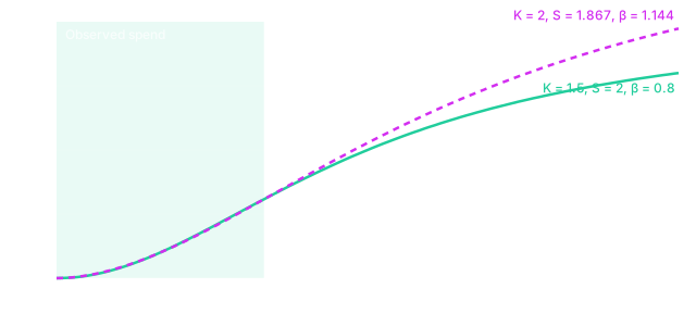
In practice, I’d treat S-curves as something the data needs to earn. If you have periods of genuinely low spend (a channel launch, a dark period, a geo test where some regions got nothing), an S-curve can be estimated. If you don’t, a concave curve is the more honest default, and the choice between them should come with a sensitivity check rather than a shrug.
Logistic, exponential and Michaelis-Menten curves
The Hill function isn’t the only option, and the tools don’t all default to it. These are the families you’ll meet most often:
| Family | Formula (times β) | Half-saturation | Where you’ll see it |
|---|---|---|---|
| Hill | Meridian, Robyn, Jin et al. (2017), PyMC-Marketing’s HillSaturation | ||
| Logistic | PyMC-Marketing’s LogisticSaturation | ||
| Exponential | Older econometric models and spreadsheets | ||
| Michaelis-Menten | PyMC-Marketing’s MichaelisMentenSaturation; the course’s Northstar case |
Despite the name, PyMC-Marketing’s logistic saturation is not an S-curve: it starts at zero and is concave everywhere, and its single parameter is an efficiency rate where larger values saturate faster. Michaelis-Menten is the Hill function with S fixed at 1, and it has the same form as the “reach transformation” Jin et al. borrow from earlier Google work on how reach builds with GRPs. The exponential curve approaches its ceiling faster than either, so at the same half-saturation point it’s flatter at high spend. PyMC-Marketing also ships tanh, log and root saturations, and a log-log model gets diminishing returns a different way, by modeling elasticities rather than a ceiling.
The explorer below lets you compare them on your own numbers. Each family is set by its half-saturation spend so the curves stay roughly comparable when you switch, and the second chart shows the slope of the first, which is the marginal return.
Try turning on “Show other families fitted to the observed range”. Each dashed curve is the best fit of another family to your chosen curve, using only the spend you marked as observed. Inside the green band they’re almost indistinguishable. Outside it, and especially at three times the highest observed spend, they can disagree enough to change where the breakeven point lands, which is the whole problem with extrapolating a saturation curve in one picture. With the default Hill curve and an observed range of $20k to $80k, the fitted curves all land within about 2.5 percent of the Hill curve at $50k a week, but at $240k the Hill curve predicts about $267k of response while a Michaelis-Menten curve fitted to the same range predicts about $394k.
Marginal return vs average return
The two numbers people most often confuse come from the same curve. Average return (often reported as ROAS or ROI) divides the channel’s total modeled contribution by its total spend, so it answers “was the money we spent worth it overall?”. Marginal return is the slope of the curve at the current spend, so it answers “what would the next dollar add?”. On any saturating curve the marginal return is below the average, because the average still includes the cheap early dollars.
The course’s lesson on saturation uses a Michaelis-Menten curve with a maximum of £100k and a half-saturation point of £40k (in the invented Northstar case). Moving from £40k to £60k of spend adds £10k of modeled revenue; moving from £160k to £180k adds about £1.82k. The response is still going up in both cases, so earlier spend hasn’t stopped working. What’s changed is how much an extra £20k buys at that level, and that’s why a channel with a strong historical ROAS can still be the wrong place for the next pound.
This is also where the breakeven threshold in the widget comes from. If your contribution margin is 40 percent, a dollar of revenue is worth 40 cents of profit, so a marginal ROAS below 2.5 loses money on the last dollar even if the average ROAS looks healthy. The marginal ROAS page goes deeper on reading the two numbers, and breakeven ROAS covers how to set the threshold from your margins. Meridian reports both ROI and marginal ROI for exactly this reason.
How saturation curves behave outside your data
A response curve can be drawn from zero to infinity, but the data only supports the part you’ve observed. The course lesson on extrapolation uses a Northstar channel that has mostly spent between £20,000 and £80,000 a week, with a planning chart extending the curve to £250,000. The software will draw that line without complaint. Within the observed range, the curve is pinned down by actual weeks of spend and sales; well outside it, the shape comes mostly from the functional form, the priors and the assumption that the audience, prices and creative will stay the same as the budget triples.
That doesn’t mean extrapolation is forbidden, but it does mean the assumptions behind it should be visible. A few habits help. Mark three spend levels on the chart: the historical range, the current level and the proposed level. Ask whether another defensible curve family would give a different answer at the proposed budget (the widget’s “other families” toggle does exactly this). Remember that parameter uncertainty within one model, which a Bayesian posterior will show you, is not the same as uncertainty about the model form or about whether the market changes when you scale. And if the recommendation relies on a region you’ve never spent in, make it a staged move with an incrementality test attached, and agree in advance what result would justify the next step.
Estimating a saturation curve you can defend
The estimation itself is usually done jointly with adstock, since both transform the same variable, and the order matters: Jin et al., Meridian and Robyn all apply adstock first and saturation second by default, so the curve describes accumulated media pressure rather than a single week’s spend (the adstock page covers when the reverse makes sense). In a Bayesian MMM you put priors on the half-saturation point and the shape; in Robyn the hyperparameter search explores alpha and gamma inside their bounds. Either way, the half-saturation point is the parameter most likely to be poorly identified when spend hasn’t varied much, so check how much the posterior moved from the prior.
The most useful single check I know is to vary the curve and see what happens to the decision, rather than to the fit. If a Hill curve, a Michaelis-Menten curve and a logistic curve all fit about equally well but recommend very different budgets, the data hasn’t answered the question yet, and the honest output is a range plus a test. These are the questions I’d ask of any response curve before it goes into a plan:
If you want to practise this on a full case, the Vexpower MMM course has lessons on saturation and extrapolation built around the invented Northstar brand, and the pillar guide to marketing mix modeling shows where the saturation curve fits in the rest of the model. For the planning side, MMM scenario planning covers how to compare budgets once you’ve got curves you trust.
